Trackernet: The Victoria Line

I’ve been meaning to look at TfL’s Trackernet API for a while now. It works through a REST based web service which gives access to all the London Underground running boards on a line by line basis. You issue an http request of the form:

http://cloud.tfl.gov.uk/TrackerNet/PredictionSummary/V

and the result is an XML file containing train information for every station on the Victoria Line. Substitute “B” instead of “V” and you get the Bakerloo line instead. I had managed to figure out a way to get approximate train locations when the Victoria Line got suspended one morning, so I couldn’t resist looking to see where all the trains had ended up:

According to my data, there are 25 trains on the line. The way the positions are calculated is quite complicated as the original information comes from the running boards for every station and the time to platform estimates. Trains are uniquely identified through a train number and a set number as a composite key. I simply iterate through all the data for every station and take the lowest time to station for every train, which gives me the train’s next station. Then I use the location code provided by the API and the time to station estimate to interpolate between the last station and the next station.

One feature worth noting is that because the time to station is given for every station along the train’s whole route, you can use the data to build up a dataset of the time required to travel between any pair of stations. Also, because the information is processed from the running boards, the program should be able to process National Rail train locations from the information on their website.

By using only the information provided in the XML response from the API means that I am able to construct a web service that doesn’t require any state information to be retained between calls. In addition to this, it doesn’t require any knowledge of the tube network and how the stations are connected together.

This is still very much a prototype, but once it’s working for all the lines, it will be released as a real-time feed on MapTube.

Extracting Data from PDFs: Clean Air in Schools

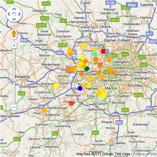
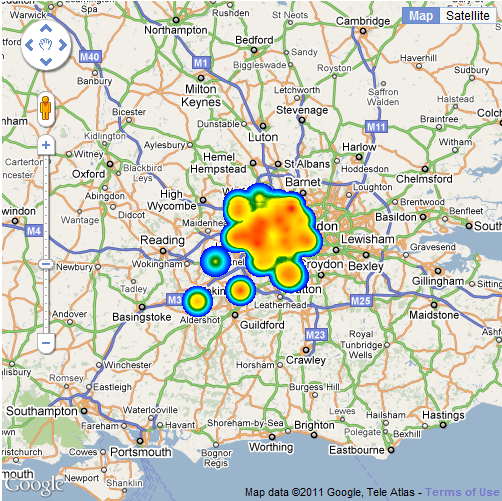
A lot of the maps I have created over the last few years have started out as tabular data in PDF documents. A recent BBC London report contained a dataset obtained from TfL of all the schools in London which are within 150 metres of a road carrying 10,000 vehicles a day or more. The report is a PDF with 21 pages, so editing this manually wasn’t an option and I decided that it was time to look into automatic extraction of tabular data from PDFs. What follows explains how I achieved this, but to start with, here is the final map of the data:

The data for the above map comes from a freedom of information request made to TfL requesting a list London schools near major roads. The request was made by the Clean Air in London group and lists all schools within 150 metres of roads carrying 10,000 vehicles a day or more. The report included a download link to the data, which is in the form of a 21 page PDF table containing the coordinates of the schools:

BBC London Article: http://www.bbc.co.uk/news/uk-england-london-13847843

Download Link to Data:  http://downloads.bbc.co.uk/london/pdf/london_schools_air_quality.pdf

The reason that PDFs are hard to handle is that there is no hard structure to the information contained in the document. The PDF language is simply a markup for placing text on a page, and so only contains information about how and where to render characters. The full PDF 1.4 specification can be found at the following link:

http://partners.adobe.com/public/developer/en/pdf/PDFReference.pdf

Extracting the data from this file manually isn’t an option, so I had a look at a library called iTextSharp (http://sourceforge.net/projects/itextsharp/), which is a port of the Java iText library into C#. The Apache PDFBox (http://pdfbox.apache.org/ ) project also looked interesting, but I went with iTextSharp for the first experiment. As the original is in Java, so are all the examples, but it’s not hard to understand how to use it. Fairly quickly, I had the following code:

[csharp]
using System;
using System.Text;
using System.IO;

using iTextSharp.text;
using iTextSharp.text.pdf;
using iTextSharp.text.pdf.parser;

namespace PDFReader
{
class Program
{
static void Main(string[] args)
{
ReadPdfFile("..\\..\\data\\london_schools_air_quality.pdf","london_schools_air_quality.csv");
}

public static void ReadPdfFile(string SrcFilename,string DestFilename)
{
using (StreamWriter writer = new StreamWriter(DestFilename,false,Encoding.UTF8))
{
PdfReader reader = new PdfReader(SrcFilename);
for (int page = 1; page {
ITextExtractionStrategy its = new iTextSharp.text.pdf.parser.SimpleTextExtractionStrategy();
//ITextExtractionStrategy its = new CSVTextExtractionStrategy();
string PageCSVText = PdfTextExtractor.GetTextFromPage(reader, page, its);
System.Diagnostics.Debug.WriteLine(PageCSVText);
writer.WriteLine(PageCSVText);
}
reader.Close();
writer.Flush();
writer.Close();
}
}
}
}
[/csharp]

This is one of the iText examples to extract all the text from a PDF and write out a plain text document. The key to extracting the data from the PDF table in the schools air quality document is to write a new class implementing the ITextExtractionStrategy interface to extract the columns and write out lines of data in CSV format.

It should be obvious from the above code that the commented out line is where I have substituted the supplied text extraction strategy class for my own one which I modified to write CSV lines:

[csharp]
ITextExtractionStrategy its = new CSVTextExtractionStrategy();
[/csharp]

The CSVTextExtractionStrategy class is defined in a separate file and is part of my “PDFReader” namespace, not “iTextSharp.text.pdf.parser”.

[csharp]
using System;
using System.Text;

using iTextSharp.text;
using iTextSharp.text.pdf;
using iTextSharp.text.pdf.parser;

namespace PDFReader
{
public class CSVTextExtractionStrategy : ITextExtractionStrategy
{
private Vector lastStart;
private Vector lastEnd;
private StringBuilder result = new StringBuilder(); //used to store the resulting string

public CSVTextExtractionStrategy()
{
}

public void BeginTextBlock()
{
}

public void EndTextBlock()
{
}

public String GetResultantText()
{
return result.ToString();
}

/**
* Captures text using a simplified algorithm for inserting hard returns and spaces
* @param renderInfo render info
*/
public void RenderText(TextRenderInfo renderInfo)
{
bool firstRender = result.Length == 0;
bool hardReturn = false;

LineSegment segment = renderInfo.GetBaseline();
Vector start = segment.GetStartPoint();
Vector end = segment.GetEndPoint();

if (!firstRender)
{
Vector x0 = start;
Vector x1 = lastStart;
Vector x2 = lastEnd;

// see http://mathworld.wolfram.com/Point-LineDistance2-Dimensional.html
float dist = (x2.Subtract(x1)).Cross((x1.Subtract(x0))).LengthSquared / x2.Subtract(x1).LengthSquared;

float sameLineThreshold = 1f; // we should probably base this on the current font metrics, but 1 pt seems to be sufficient for the time being
if (dist > sameLineThreshold)
hardReturn = true;

// Note: Technically, we should check both the start and end positions, in case the angle of the text changed without any displacement
// but this sort of thing probably doesn’t happen much in reality, so we’ll leave it alone for now
}

if (hardReturn)
{
//System.out.Println("<< Hard Return >>");
result.Append(Environment.NewLine);
}
else if (!firstRender)
{
if (result[result.Length – 1] != ‘ ‘ && renderInfo.GetText().Length > 0 && renderInfo.GetText()[0] != ‘ ‘)
{ // we only insert a blank space if the trailing character of the previous string wasn’t a space, and the leading character of the current string isn’t a space
float spacing = lastEnd.Subtract(start).Length;
if (spacing > renderInfo.GetSingleSpaceWidth() / 2f)
{
result.Append(‘,’);
//System.out.Println("Inserting implied space before ‘" + renderInfo.GetText() + "’");
}
}
}
else
{
//System.out.Println("Displaying first string of content ‘" + text + "’ :: x1 = " + x1);
}

//System.out.Println("[" + renderInfo.GetStartPoint() + "]->[" + renderInfo.GetEndPoint() + "] " + renderInfo.GetText());
//strings can be rendered in contiguous bits, so check last character for " and remove it if we need
//to stick two rendered strings together to form one string in the output
if ((!firstRender)&&(result[result.Length – 1] == ‘\"’))
{
result.Remove(result.Length – 1, 1);
result.Append(renderInfo.GetText() + "\"");
}
else
{
result.Append("\"" + renderInfo.GetText() + "\"");
}

lastStart = start;
lastEnd = end;
}

public void RenderImage(ImageRenderInfo renderInfo)
{
}
}
}
[/csharp]

As you can probably see, this file is based on “iTextSharp.text.pdf.parser.SimpleTextExtractionStrategy”, but inserts commas between blocks of text that have gaps between them. It might seem like a better idea to parse the structure of the PDF document and write out blocks of text as they are discovered, but this doesn’t work. The London schools air quality example had numerous instances where text in one of the cells (e.g. a school name, Northing or Easting) was split across two text blocks in the pdf file. The only solution is to implement a PDF renderer and extract text using its positioning on the page to separate columns.

The result of running this program on the London schools air quality PDF is a nicely formatted CSV file which took about 5 minutes to edit into a format that I could make the map from. All I had to do was remove the page number and title lines from between the pages and add a header line to label the columns. There were also a couple of mistakes in the original PDF where the easting and northing had slipped a column.

Two Line Elements

Prompted by the final space shuttle launch of Atlantis, I thought I would have another look at two line elements (TLEs). These are coded lines of data that describe the orbital dynamics of a space vehicle. The last time I looked at this was when I was working on a GPS tracking project and we wanted to predict the satellite constellation at a particular time of day, but TLEs can also be downloaded for the shuttle and International Space Station.

NASA’s J-Track shows the shuttle and ISS in near real-time:  http://spaceflight.nasa.gov/realdata/tracking/index.html

Image Copyright NASA

The TLE for the shuttle can be downloaded from the following link:

http://spaceflight.nasa.gov/realdata/sightings/SSapplications/Post/JavaSSOP/orbit/SHUTTLE/SVPOST.html

The mathematics to calculate a position from the TLE is published in the NORAD paper entitled “Spacetrack Report Number 3” (1980/1988). A later revision to this paper is also publicly available and there are various ports of the algorithm from Fortran into C, C++ and C#. While investigating this, I stumbled across a very useful library written by Michael F. Henry. It’s called “OrbitTools” and is a C++ and C# (both managed .net) implementation. His download page contains lots of other useful information and links to the spacetrack revised paper:

http://www.zeptomoby.com/satellites/

The next step was to download his C# library and write the code to load the shuttle TLE and convert the position to a location on the Earth. One point worth mentioning here is that the library calculates lat/lons in WGS72 rather than WGS84. The spheroids are slightly different, so there will be some small accuray issues, but it’s close enough for our purposes.

Having downloaded and included the OrbitTools library into a new C# project, the code to calculate the shuttle position is as follows:

[csharp]
const string TleTitle = "SHUTTLE";
const string Tle1 = "1 37736U 11031A 11190.45039996 .00020000 00000-0 20000-3 0 9019";
const string Tle2 = "2 37736 51.6412 48.9000 0077926 223.8647 135.6325 16.00701051 142";

//DateTime dt = DateTime.UtcNow;
DateTime dt = new DateTime(2011, 7, 9, 10, 40, 18, DateTimeKind.Utc);

Tle VehicleTle = new Tle(TleTitle, Tle1, Tle2);
Orbit VehicleOrbit = new Orbit(VehicleTle);
TimeSpan ts = VehicleOrbit.TPlusEpoch(dt); //how old is our TLE?
Eci VehicleEci = VehicleOrbit.GetPosition(dt); //OK, they want GMT, not UTC
CoordGeo VehicleGeoCoord = VehicleEci.ToGeo();
double lat = VehicleGeoCoord.Latitude*180.0/Math.PI;
double lon = VehicleGeoCoord.Longitude*180.0/Math.PI;
double alt = VehicleGeoCoord.Altitude;
if (lon > 180.0f) lon = -(360.0f – lon);
Console.WriteLine(TleTitle+": lat=" + lat + " lon=" + lon + " alt=" + alt);
[/csharp]

When this is run, the result written to the console is as follows (apologies for the unnecessary precision, but that’s the output I get):

lat=-25.316480642262878 lon=-60.024030447329437 alt=291.32191224312828

These values are very close to the figures on NASA’s J-Track image reproduced earlier, so we’re close to the official coordinates. When repeating this, it’s important to fix the time in the code to the same time as displayed on the J-Track applet and not just use “DateTime.UtcNow” as is commented out in the code. This is one source of inaccuracy as we’re assuming the position was calculated at zero milliseconds, which might not be the case.

References and Links

NASA J-Track: http://spaceflight.nasa.gov/realdata/tracking/index.html

OrbitTools C++/C# SGP4/SDP4 Library and other information: http://www.zeptomoby.com/satellites/

TLE Data for STS 135: http://spaceflight.nasa.gov/realdata/sightings/SSapplications/Post/JavaSSOP/orbit/SHUTTLE/SVPOST.html

Original Spacetrack Report Number 3 (1980): http://www.celestrak.com/NORAD/documentation/spacetrk.pdf

Spacetrack Report Number 3 Revisited: http://www.celestrak.com/publications/AIAA/2006-6753/

Other sources of TLE data: http://celestrak.com/NORAD/elements/

Weather Underground

I’ve been looking at the Weather Underground API (http://wiki.wunderground.com/index.php/API_-_XML) which gives access to the observation stations and the data they are collecting.

All the stations returned from the Weather Underground XML API when using "London" as the search string. Colour indicates air temperature with blue=12.7C, green=13.9C and red=20.5C

The API uses simple commands to query for a list of stations, for example:

http://api.wunderground.com/auto/wui/geo/GeoLookupXML/index.xml?query=london,united+kingdom

Using C# and .net, this is accomplished as follows:
[csharp] WebRequest request = WebRequest.Create(string.Format(GeoLookupXML, @"london,united+kingdom"));
HttpWebResponse response = (HttpWebResponse)request.GetResponse();
XmlDocument doc = new XmlDocument();
doc.Load(response.GetResponseStream());[/csharp]
Then the returned XML document is parsed using XQuery to extract the station name, lat/lon coordinates and whether it is an ICAO station or a personal weather station.
[csharp]XmlNodeList Stations = doc.GetElementsByTagName("station");
foreach (XmlNode Station in Stations)
{
XmlNode IdNode = Station.SelectSingleNode("id");
XmlNode ICAONode = Station.SelectSingleNode("icao");
}[/csharp]
This gets us a list of stations ids and ICAOs which can then be used to build individual queries to obtain real time data from every station:
[csharp]foreach (string Id in PWSStations)
{
XmlDocument ob = GetCurrentPWSOb(Id);
XmlNode Ntime = ob.SelectSingleNode(@"current_observation/observation_time_rfc822");
XmlNode Nlat = ob.SelectSingleNode(@"current_observation/location/latitude");
XmlNode Nlon = ob.SelectSingleNode(@"current_observation/location/longitude");
XmlNode NairtempC = ob.SelectSingleNode(@"current_observation/temp_c");
string time = Ntime.FirstChild.Value;
string airtempC = NairtempC.FirstChild.Value;
string lat = Nlat.FirstChild.Value;
string lon = Nlon.FirstChild.Value;

//do something with the data…
}

//NOTE: only slight difference in xml format between PWS and ICAO
foreach (string ICAO in ICAOStations)
{
XmlDocument ob = GetCurrentICAO(ICAO);
XmlNode Ntime = ob.SelectSingleNode(@"current_observation/observation_time_rfc822");
XmlNode Nlat = ob.SelectSingleNode(@"current_observation/observation_location/latitude");
XmlNode Nlon = ob.SelectSingleNode(@"current_observation/observation_location/longitude");
XmlNode NairtempC = ob.SelectSingleNode(@"current_observation/temp_c");
string time = Ntime.FirstChild.Value;
string airtempC = NairtempC.FirstChild.Value;
string lat = Nlat.FirstChild.Value;
string lon = Nlon.FirstChild.Value;

//do something with the data…

}[/csharp]
After that it’s simply a matter of writing all the data to a CSV file so that you can do something with it.

Air temperature for London plotted using the MapTubeD heatmap tile renderer

Genesis: How to Build a Planet

John Conway’s “Game of Life” was one of the first things I ever wrote in Java, back in the days when we were using 1.1. This is a slight variation on the traditional 2D view, where the alife simulation is wrapped around a spinning globe. The results are shown below, along with the link to the web page containing the applet.
Conways Game of Life
Conway's Game of Life

 http://www.casa.ucl.ac.uk/richard/demos/planet/GameOfLifePlanet.html

The way this was created was as follows:

Step 1 – Create the Planet Mesh

I’ve defined my axes with x to the right, z up and y into the screen. This is slightly unusual, but maps to the ground plane which was originally XZ.

for z=0 to numZ-1
    for x=0 to numX-1
          ax=x/numX*2.0*PI-PI;
          az=z/numZ*PI-PI/2;
          cx=radius*cos(az)*sin(ax);
          cy=radius*cos(az)*cos(ax);
          cz=radius*sin(az);
          coords[x][z]=new Point3D(cx,cy,cz);

The mesh of points can be wrapped around in the x direction, but not Z, so we need an extra line of points at the South pole. I’ve also taken the radius to be 1.0 as using the unit sphere simplifies a lot of the graphics calculations that follow.

This gives you the following result:

Planet Mesh
Planet Mesh

Step 2 – Spin the World

Next I added an animation thread that increments ‘A’, the angle of rotation of the planet. In the rendering code for the mesh I rotate the points to spin the planet around the poles. The interesting thing here is that you don’t need the Y coordinate as there’s no projection, so that saves a few operations.

xp[i]=radius*(xpoints[i]*cos(A)+ypoints[i]*sin(A))
//yp[i]=radius*(xpoints[i]*sin(A)-ypoints[i]*cos(A))
zp[i]=radius*zpoints[i] 

The back faces have been removed by using the direction between the surface normal and the viewer. Any face pointing away from the viewer is not drawn.

Step 3 – Add the Game of Life Simulation

I already had an implementaion of this in Java, so I just pulled it into the project. The following wikipedia article contains everything you could every need to know about Conway’s Game of Life:

http://en.wikipedia.org/wiki/Conway’s_Game_of_Life

Then it’s just a case of running the ALife simulation and linking the output to the cells in the planet mesh. The grid used for the Game of Life simulation and the mesh making up the planet are the same size, so there is a simple one to one relationship.

Game of Life Planet
Game of Life Planet


Step 4 – Lights

To improve the realism, I added some lighting using Lambert’s cosine rule. The direction of the light is [-1.0, 0.0, 0.0] which makes the intensity calculation straightforward. The light is assumed to be far enough away that the direction of the light is constant over the whole object. The planet is a unit sphere centred on the origin, so the normal to the surface patch is just a ray through the origin and the centre of the patch. I’ve actually taken the top left corner to save having to calculate the centre point, but it doesn’t make much difference to the effect.

According to Lambert’s cosine rule, the intensity of the patch is proportional to the cosine of the angle between the surface normal and the light. We use the dot product of the two vectors to get the cosine of the acute angle between them. As both vectors are already normalised beforehand, we don’t have to normalise them ourselves.

In this view, any game of life cell that is ‘on’ is drawn in blue, while any that are ‘off’ are white. The white colour uses the diffuse lighting while the blue is drawn as emissive so you can see the patterns as they go around the dark side of the globe. I’ve also added a line at the 0 and 180 degree longitude positions so you can see the planet rotating.

Here is an image of a “Gosper Glider Gun” about to shoot gliders at itself from around the other side of the planet. The applet link below contains a number of the more common patterns.

Next Steps:
The mapping of the life grid to the planet mesh could do with some improvement. Anything moving east or west maps around the sphere correctly, but anything moving through the north pole reappears at the south and vice-versa. There are better ways to map grids onto spheres, but that’s for next time. I also have an erosion-based model that I wrote a long time ago to create realistic looking land and water masses, which this was was originally intended for.

Downloadable Preview – GENeSIS Exhibition Space

The following exhibition space is a proof of concept, looking at the ability to share and display city datasets and simulations within an interactive game engine. Available for download on both the PC and Mac (intel) platforms the space is the result of a few days work with the Unity Engine, it is intended to be viewed in the spirit of development rather than a completed product.

The room includes our first ‘crowd and delegate’ models direct from 3D Max, created as basic wander and avoid simulations they provide the building blocks of emergent behaviour within the cityscape.

City wide data sets can to be honest be very ‘dry’, the whole point of digital urban is to look at new ways to outreach, visualise and ultimately communicate urban data. The ability to include 3D models via ESRI ArcScene is a notable step forward, pictured below is the retail and office space in London measured on a 500m grid. We note some polygon issues here but these are known and we think we have a way to fix them – its to do with the way ArcScene exports, the model forms the centre of the exhibition space:

The room features various architectural models, including the Swiss Re building and the GLA in London, it also features a number of our latest output movies, the London LiDAR and Second Life Agents are of particular note.

The model is, as we mentioned, proof of concept, the next step is the addition of themed rooms and a more organised structure. We think the concept of virtual exhibition spaces is a strong one, so as ever any comments are most welcome…

Download the model for Windows XP/Visa (221 Mb zip file)

Unzip the file, open the folders and run the .exe file.

Download the model for Mac (222 Mb zip file)

Extract and simply run the .dmg file.

Use the mouse to look around, W/S move forwards/backwards, Space to jump.

GENeSIS Exhibition Space

We have spent the last few days giving the game engine Unity a spin. The pro version has various additions to the lower cost indie edition, most notably for our use the ability to import movies as textures and use dynamic shadows. Our movie below provides an update on progress:

Unity: Creating a City Exhibition Space – Update 2 from digitalurban on Vimeo.

The aim is to create an exhibition space exploring simulation and the city… more to follow.

ESRC Seminar Series: Microsimulation Modelling

Four seminars will be held over the spring and summer of 2009 which will provide an opportunity to evaluate the state of play and research opportunities in the field.  The first two seminars will be held in London on April 2nd and May 6th, and the others in Leeds (July 2nd) and Brighton (September 16th).  The full programme is shown below.�
The first seminar deals with the theme of ‘scaling up, scaling down’.  Major speakers include Neil Ferguson (Imperial College) and Holly Sutherland (University of Essex).  There will also be contributions on the MoSeS dynamic model, and on the GENeSIS e-infrastructure.  The second seminar on the theme of ‘adding behaviour’  looks of particular interest to the GENeSIS community.  The presenters include Edmund Chattoe-Brown (co-investigator of the SIMIAN project), Gary Polhill (Macauley Institute) and our own Alison Heppenstall.  Seminar 3 is concerned with land-use and transportation modelling, while the final seminar will adopt a more agenda-setting theme.
The series is organised by Dr Paul Williamson (University of Liverpool) .   Paul began his academic career at Leeds working with Phil Rees on problems relating to simulation and the delivery of social care.  His work on the development and evaluation of simulation algorithms is particularly well-regarded (Williamson et al, 1998; Voas and Williamson, 2001).  Paul has also written on the theme of geodemographics:  another  heavily cited paper with David Voas highlights the spatial diversity which is typically assumed away by  geodemographic classifications ).  Paul Williamson is editor of the International Journal of Microsimulation.


ESRC Seminar Series ‘Microsimulation modelling in the UK: bridging the gaps’


A short series of four closely-spaced seminars designed to:

Identify and agree common areas of challenge
Encourage greater/more


  • pooling of effort
  • sharing of existing solutions
  • collaborative research grant applications
Planned programme

Seminar 1 ‘Scaling up; scaling down’


Thursday 2nd April; London
Invited speaker / Team


Prof Neil Ferguson (Imperial)  

Large scale modelling of flu epidemics  

James Carpenter (LSHTM)  

Bootstrapping and multiple imputation  

Holly Sutherland / EUROMOD  

Flexing to add more countries/tax-benefit systems  

Mark Birkin / MOSES  

GRID/parallel computing  

Mark Birkin / MOSES  

Dealing with migration in sub-national dynamic msms  

Chris Drane / DWP  

Bigger vs. faster  

Paul Williamson (Liverpool)  

Creating synthetic sub-regional baseline populations  

Seminar 2 ‘Adding Behaviour’ 

Wednesday 6th May; London
Invited speaker / Team


Topic


Prof Alan Duncan (Nottingham)  

Economic behavioural response:state of the art  

DWP / IFS  

Economic behavioural response: practical challenges  

Mike Murphy (MAP2030)  

Modelling kinship  

Ruth Hancock (MAP2030)  

Modelling demand for care  

Edmund Chattoe-Brown  

Agent-based modelling  

Alison Heppenstall  

Agent-based modelling  

Gary Polhill / FEARLUS  

Modelling evolving patterns of land-use  

Seminar 3 ‘Moving beyond tax-benefit and demographic modelling’


Thursday 2nd July; Leeds
Inivited speaker / team


Topic


SParamics  

Transport microsimulation  

Kai Nagel (Berlin)  

Transport microsimulation  

David Simmonds  

Transport microsimulation  

Ben Anderson / Chimera  

Retail / expenditure  

Dimitris Ballas (Sheffield)  

Happiness  

David Bell (Stirling)  

Demand for care  

Gary Polhill / FEARLUS  

Modelling evolving patterns of land-use  


Seminar 4 ‘Bridging the gaps’ / ‘Setting the agenda’


Friday 11th September; Brighton (as part of BSPS annual conference)
Invited speaker / team


Topic


NATSEM


How to build a coherent national msm effort


Statistics Canada


How to build a coherent national msm effort


MAP2030


What we are doing; what we can share; where next?


SAGE


Ditto


EUROMOD


Ditto


MOSES


Ditto


DWP


Ditto


HMRC


Ditto


IFS


Ditto


Sheffield


Ditto


Liverpool


Ditto


Aberdeen


Ditto


The London Database

A quick update as we have been working on a number of projects. One is creating a simplified road network for London to explore the road structure in relation to network theory (see Masucci) but also for its use in accessibility measures. Our second project is building a detailed land use database for London (using SQL Server which we access through ArcSDE).

The purpose of the database is so our research group can use it for various applications (such as land use modelling, residential agent-based modelling, urban sprawl analysis, sustainability, rain water harvesting etc). The aim of the land use database is to tag all the buildings within London with various attributes such as use, whether it is a house, a flat or an office etc. The data sets we are using include; Ordnance Survey MasterMap and Address layer 2 , building heights via LIDAR data from InfoTerra. We are using Cities Revealed data for residential building types and age along with several other datasets. When combined it will allow for fine scale and extensive modelling of the of London’s housing market & built environment.

Below are some preliminary outputs, including a land use visualisation of the Isle of Dogs, the London Borough of Tower Hamlets broken down by residential property types and finally residential density within a section of the Isle of Dogs.

Isle of Dogs Land-use 3D Visualisation (Red is Residential, Dark blue is Office, Light blue is Office Mixed Use).

Housing Classification of Tower Hamlets, London (yellow is terraced housing, blue is flats and grey is non residential).

Residential Density within the Isle of Dogs (Dwellings per Hectare)

GENeSIS History

This is a short history of our cooperation through the National Centre for e-Social Science


From 2005, two of the key research nodes of NCeSS were located in London at UCL – GeoVUE and at Leeds in the University of Leeds – MoSeS. GeoVUE ended on the 30th September 2008 and GENeSIS began on 1st October 2008. This is a convenient point to explain all these terms. GeoVUE stands for Geographic Virtual Urban Environments. It was a project which essentially developed web-based services for the visualisation of 2D maps producing in particular GMapCreator and MapTube amongst other software for map mashup and then moved on to consider importing 2D maps and related geospatial data into 3D environment, specifically games and virtual worlds but also 3D GIS, CAD and 3D virtual globes.


GENeSIS is a little different in that it stands for GENerative e-SocIal Science. The acronym like all good symbols for research projects can be unpacked in diverse ways which emphasise our focus on space and simulation but we consider the previous statements the baseline definition. It joins GeoVUE to MoSeS which is the project that the Leeds node has developed in the first phase of NCeSS funding. MoSeS is a microsimulation model of the UK economy developed using microsimulation logics and applied to subdivisions of the UK space at different spatial scales. It is used for policy analysis such as the impact of aging on public services. MoSeS stands for MOdelling and Simulation for e-Social Science.


GENeSIS (= GeoVUE + MoSeS) is to develop microsimulation models for social science and to link these to the emerging paradigm of agent-based models. The UCL node will develop ABMS and their visualisation while the Leeds node will link microsimulation to ABMs. Model development and visualisation will take place in both nodes and the programme of research will be integrated. A rudimentary web site has been set up (http://www.genesis.ucl.ac.uk/) but we consider that this blog will take over as our basic web presence, once we have experimented with formats.


Mike Batty, CASA, UCL