Trackernet: Where are all the Tube Trains?

This is starting to become obsessive, but I can’t help wondering how many trains are running on the London Underground and where they all are. The Trackernet web service released by TfL allows you to see all the running boards for stations on a line, but doesn’t tell you where all the trains are. I did an earlier post about just the Victoria line trains, but I’ve now built this into a web service that works out locations for trains on the whole network.


Trains on the London Underground network for 11:30am on 30th November 2011

The map colours follow the normal line colours, so District (Green), Victoria (Light Blue), Central (Red), Northern (Black), Bakerloo (Brown), Jubilee (Grey), Piccadilly (Dark Blue), Waterloo and City (light green). Note that Circle and Hammersmith and City are all shown as yellow and there are no pink markers on the map. This is because the Trackernet API does not distinguish between Circle and Hammersmith and City trains and both lines are queried in one web request, so they’re difficult to separate out.

The idea is to build this into a web service and publish it on MapTube as a real-time Tube map. Using the locations of trains and the time to station information we can build a model of whether a line is running normally and where delays are occurring.

The basic technique behind how the positions are calculated relies on using the time to station information from the running boards at every station on the route to find the minimum time for every unique train. This is then taken as the most accurate location estimate and its position interpolated between the last and next stations based on the time. It is actually a lot harder to work out which line a train is on due to the fact that multiple lines can share platforms at the same station. For example, query the Piccadilly line and the District line and the resulting data will contain Barons Court for both, so you have to separate out the Piccadilly trains and the District trains and make sure you don’t count the same ones twice.

Now that the code can handle the Underground network, the next steps are to do the same for National Rail, London Buses and London River Services.

If you’re interested in live train data, it’s also worth looking at the following site that was created by Matthew Somerville: http://traintimes.org.uk/map/tube

FBX Exporters Part 4

In the previous three parts, I outlined the plan for getting geometry from MapTube via C Sharp into an FBX file using the C++ SDK provided by Autodesk. This final part shows data in a world map exported from MapTube and imported into 3DS Max.

The above image shows the world countries 2010 outline from MapTube. There a few countries missing as there was no data for them in the original dataset, so they show as blank on a MapTube map and their geometry is not exported. This is more visible in the perspective view where you can see the holes in Africa and the Middle East:

The exported geometry will eventually be coloured in the same way as MapTube, but for the moment all the geometry objects have a green material assigned to them.

The final export file can be downloaded from the following link: MyFBXExport


It’s worth pointing out that I’ve had a number of problems with the Quicktime FBX plugin that comes with the Autodesk FBX SDK. It seems to crash every time I close it and when displaying the above file there are some significant problems with how it renders the geometry. Most notably around the Hudson Bay area in Canada, parts of Europe and much of Russia. As it displays fine in Max, I can only assume this is a limitation of the Quicktime FBX renderer. I’ve also had to do some re-scaling of the geometry as it is exported in the Google Mercator projection, using metres. This means that the numbers are too big for Max to handle, so I’ve had to rescale them.

To recap on how this process works, here are the development steps needed to achieve it:

1. A C Sharp program which is a modification of the MapTubeD tile rendering procedure reads the geometry and data from the MapTube server and returns it as an iteration of SqlGeometry objects.

2. Each SqlGeometry object is simplified using the Reduce operation as we don’t need the full level of detail in the output FBX file.

3. The C Sharp program uses native methods in a C++ DLL, which I’ve written to control the operation of the FBX exporter in Autodesk’s SDK. A handle to the FBX document and scene that we want to create is obtained and then a native “AddGeometry” function is used on every geometry object until a final “WriteFile” function is called. The geometry is passed using the OGC well known binary format which is an efficient way of passing large blocks of complex geometry and is also independent of byte ordering.

The DLL which does the actual export is a 32 bit program with functions exported using C names rather than decorated C++ names to make it easy to link to the C Sharp function stubs. Internally, I’m using the GEOS library to parse the well known binary geometry, extract polygons and write the points to the FBX scene hierarchy.

That’s the proof of concept to demonstrate that this method works. The aim now is to see what we can do with geographic data now that we have the ability to load it into art tools like Max and Maya, game engines like Unity, or frameworks like XNA.


FBX Exporters Part 2

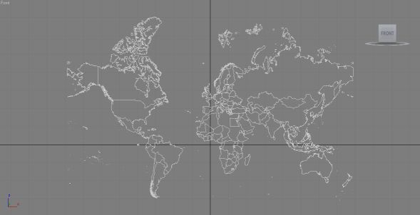
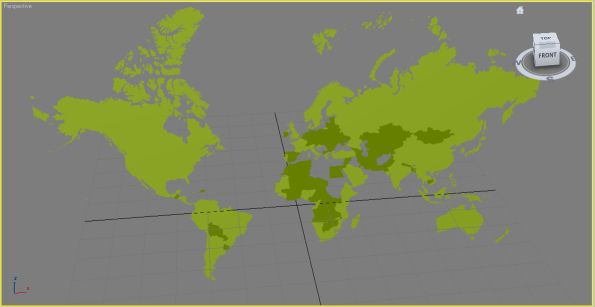
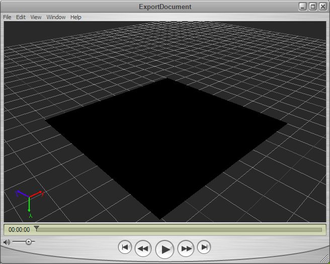
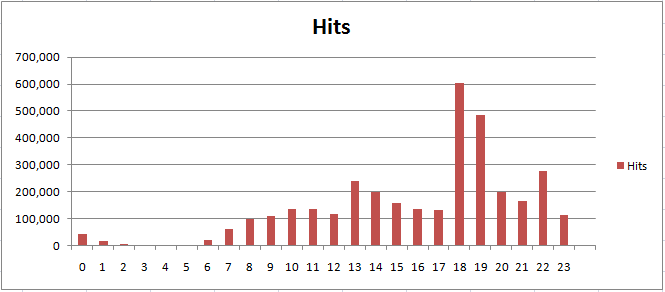
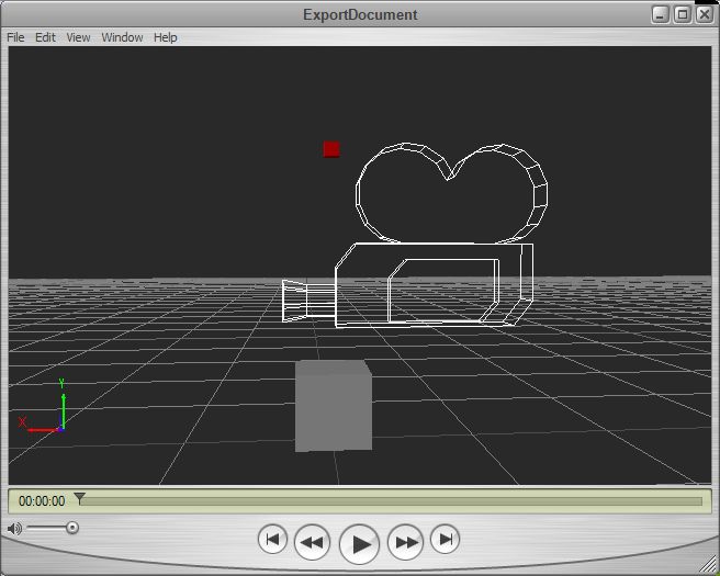
In the first FBX exporter post I got to the point where the export of simple geometry from one of the Autodesk SDK examples could be loaded by the Quicktime plugin. This used the SDK as a multithreaded statically linked library which I used with one of the examples to create a plane object. The following image shows a more complicated file containing a marker (red), custom geometry in the form of a cube (grey) and a camera (looks like a camera).

The code to get to this point is rather complicated, but I copied the UI Examples CubeCreator example program supplied with the SDK which showed how to set up the cube mesh with all the correct normals and textures.

The scene graph is set up with a camera, marker and mesh as follows:

[c language=”++”]
// build a minimum scene graph
KFbxNode* lRootNode = pScene->GetRootNode();
lRootNode->AddChild(lMarker);
lRootNode->AddChild(lCamera);
// Add the mesh node to the root node in the scene.
lRootNode->AddChild(lMeshNode);
[/c]

The creation of the mesh object prior to this is a lot more complicated:

[c language=”++”]
// Define the eight corners of the cube.
// The cube spans from
// -5 to 5 along the X axis
// 0 to 10 along the Y axis
// -5 to 5 along the Z axis
KFbxVector4 lControlPoint0(-5, 0, 5);
KFbxVector4 lControlPoint1(5, 0, 5);
KFbxVector4 lControlPoint2(5, 10, 5);
KFbxVector4 lControlPoint3(-5, 10, 5);
KFbxVector4 lControlPoint4(-5, 0, -5);
KFbxVector4 lControlPoint5(5, 0, -5);
KFbxVector4 lControlPoint6(5, 10, -5);
KFbxVector4 lControlPoint7(-5, 10, -5);

KFbxVector4 lNormalXPos(1, 0, 0);
KFbxVector4 lNormalXNeg(-1, 0, 0);
KFbxVector4 lNormalYPos(0, 1, 0);
KFbxVector4 lNormalYNeg(0, -1, 0);
KFbxVector4 lNormalZPos(0, 0, 1);
KFbxVector4 lNormalZNeg(0, 0, -1);

// Initialize the control point array of the mesh.
lMesh->InitControlPoints(24);
KFbxVector4* lControlPoints = lMesh->GetControlPoints();
// Define each face of the cube.
// Face 1
lControlPoints[0] = lControlPoint0;
lControlPoints[1] = lControlPoint1;
lControlPoints[2] = lControlPoint2;
lControlPoints[3] = lControlPoint3;
// Face 2
lControlPoints[4] = lControlPoint1;
lControlPoints[5] = lControlPoint5;
lControlPoints[6] = lControlPoint6;
lControlPoints[7] = lControlPoint2;
// Face 3
lControlPoints[8] = lControlPoint5;
lControlPoints[9] = lControlPoint4;
lControlPoints[10] = lControlPoint7;
lControlPoints[11] = lControlPoint6;
// Face 4
lControlPoints[12] = lControlPoint4;
lControlPoints[13] = lControlPoint0;
lControlPoints[14] = lControlPoint3;
lControlPoints[15] = lControlPoint7;
// Face 5
lControlPoints[16] = lControlPoint3;
lControlPoints[17] = lControlPoint2;
lControlPoints[18] = lControlPoint6;
lControlPoints[19] = lControlPoint7;
// Face 6
lControlPoints[20] = lControlPoint1;
lControlPoints[21] = lControlPoint0;
lControlPoints[22] = lControlPoint4;
lControlPoints[23] = lControlPoint5;

// We want to have one normal for each vertex (or control point),
// so we set the mapping mode to eBY_CONTROL_POINT.
KFbxGeometryElementNormal* lGeometryElementNormal= lMesh->CreateElementNormal();

lGeometryElementNormal->SetMappingMode(KFbxGeometryElement::eBY_CONTROL_POINT);

// Set the normal values for every control point.
lGeometryElementNormal->SetReferenceMode(KFbxGeometryElement::eDIRECT);

lGeometryElementNormal->GetDirectArray().Add(lNormalZPos);
lGeometryElementNormal->GetDirectArray().Add(lNormalXPos);
lGeometryElementNormal->GetDirectArray().Add(lNormalZNeg);
lGeometryElementNormal->GetDirectArray().Add(lNormalXNeg);
lGeometryElementNormal->GetDirectArray().Add(lNormalYPos);
lGeometryElementNormal->GetDirectArray().Add(lNormalYNeg);

// Array of polygon vertices.
int lPolygonVertices[] = { 0, 1, 2, 3, 4, 5, 6, 7, 8, 9, 10, 11,12, 13,
14, 15, 16, 17, 18, 19, 20, 21, 22, 23 };

// Create UV for Diffuse channel.
KFbxGeometryElementUV* lUVDiffuseElement = lMesh->CreateElementUV( "DiffuseUV");
K_ASSERT( lUVDiffuseElement != NULL);
lUVDiffuseElement->SetMappingMode(KFbxGeometryElement::eBY_POLYGON_VERTEX);
lUVDiffuseElement->SetReferenceMode(KFbxGeometryElement::eINDEX_TO_DIRECT);

KFbxVector2 lVectors0(0, 0);
KFbxVector2 lVectors1(1, 0);
KFbxVector2 lVectors2(1, 1);
KFbxVector2 lVectors3(0, 1);

lUVDiffuseElement->GetDirectArray().Add(lVectors0);
lUVDiffuseElement->GetDirectArray().Add(lVectors1);
lUVDiffuseElement->GetDirectArray().Add(lVectors2);
lUVDiffuseElement->GetDirectArray().Add(lVectors3);

//Now we have set the UVs as eINDEX_TO_DIRECT reference and in eBY_POLYGON_VERTEX mapping mode
//we must update the size of the index array.
lUVDiffuseElement->GetIndexArray().SetCount(24);

// Create polygons. Assign texture and texture UV indices.
for(int i = 0; i < 6; i++)
{
// all faces of the cube have the same texture
lMesh->BeginPolygon(-1, -1, -1, false);

for(int j = 0; j < 4; j++)
{
// Control point index
lMesh->AddPolygon(lPolygonVertices[i*4 + j]);

// update the index array of the UVs that map the texture to the face
lUVDiffuseElement->GetIndexArray().SetAt(i*4+j, j);
}

lMesh->EndPolygon();
}

[/c]

So, we have to define the vertices (control points in the language of the SDK), normals and UV coordinates for the mesh to show in the Quicktime viewer. It’s also worth mentioning that I’ve had to force the output FBX file from the exporter to be in binary format as the viewer refuses to load the ASCII format FBX. In addition to this, I’m still getting application crashes when I close the Quicktime viewer.

Now I have the ability to create custom geometry, the next step is to write an interface to allow me to pass geographic data to the exporter via C#. After giving this some thought, the obvious solution is to pass well-known binary (WKB) from the C# program to the C++ library as a block of bytes. This is a relatively easy format to produce and decode into geometry, so shouldn’t take long to write.

Part three will deal with the mechanics of getting actual geometry to the exporter and generating an FBX file from real geographic data.

Exporting Geographic Data in FBX Files

I’ve been looking at how to export the geographic information contained in a MapTube map into an art tool like 3DS Max or Maya. The reason for this is firstly to make it easier to produce high quality geographic presentations, but also, by employing a recognised art tool chain, we can also get the data into 3D visualisation systems built around XNA (XBox) or Unity.

Originally, I was going to implement a 3DS exporter as this is a well-used format that would allow geometry to be imported by Google Sketchup, Blender, or a long list of professional art tools. After coming across Autodesk’s FBX SDK, I decided to create an FBX exporter instead. Although this is a format that can’t be loaded by either Sketchup or Blender, the SDK is quite flexible and can also export Collada (DAE) and Wavefront OBJ files which the free tools can import. In addition to this, it can be imported by both Unity and XNA.

Autodesk supply a viewer plugin for Quicktime, but I had some problems getting this to work with my first export attempts. The example below shows a simple screenshot:

Although a flat black plane on a grey background isn’t fantastic for a first attempt, it took a while to get this far as the examples don’t tell you that the Quicktime viewer doesn’t like ASCII format FBX files and you have to change the example format to BINARY.

[c language=”++”]
//altered export from ASCII to Binary
int lFormatIndex, lFormatCount = pSdkManager->GetIOPluginRegistry()->GetWriterFormatCount();

for (lFormatIndex=0; lFormatIndex<lFormatCount; lFormatIndex++)
{
if (pSdkManager->GetIOPluginRegistry()->WriterIsFBX(lFormatIndex))
{
KString lDesc =pSdkManager->GetIOPluginRegistry()->GetWriterFormatDescription(lFormatIndex);
printf("%s\n",lDesc.Buffer()); //print out format strings
//char *lASCII = "ascii";
char *lBinary = "binary";
if (lDesc.Find(/*lASCII*/lBinary)>=0)
{
pFileFormat = lFormatIndex;
break;
}
}
}
[/c]

This is a copy of the “ExportDocument” example that comes with the SDK, but with the type changed to binary to allow it to load.

The next problem is learning how to create my own geometry and figuring out a way of connecting the native C++ library to the managed C# code used by MapTube. My initial thought was to create a managed wrapper for the FBX SDK and use marshalling, but, on further examination of the SDK, it’s much too complicated to do in any reasonable amount of time. So, plan B is to write the code to do the export as a native C++ process, expose enough methods to allow this to be controlled through marshalling and interop via the C# code and do the FBX export through that route. This only depends on being able to marshall the large amount of geometry data, but this should be possible to work out.

After these first experiments, it’s looking like the pattern will be something like a reader/writer object with a choice of export formats as FBX, Collada or OBJ to allow the assets to be loaded into as many art packages as possible.

The next post will cover the generation of the geometry and its export to FBX.

Trackernet: The Victoria Line

I’ve been meaning to look at TfL’s Trackernet API for a while now. It works through a REST based web service which gives access to all the London Underground running boards on a line by line basis. You issue an http request of the form:

http://cloud.tfl.gov.uk/TrackerNet/PredictionSummary/V

and the result is an XML file containing train information for every station on the Victoria Line. Substitute “B” instead of “V” and you get the Bakerloo line instead. I had managed to figure out a way to get approximate train locations when the Victoria Line got suspended one morning, so I couldn’t resist looking to see where all the trains had ended up:

According to my data, there are 25 trains on the line. The way the positions are calculated is quite complicated as the original information comes from the running boards for every station and the time to platform estimates. Trains are uniquely identified through a train number and a set number as a composite key. I simply iterate through all the data for every station and take the lowest time to station for every train, which gives me the train’s next station. Then I use the location code provided by the API and the time to station estimate to interpolate between the last station and the next station.

One feature worth noting is that because the time to station is given for every station along the train’s whole route, you can use the data to build up a dataset of the time required to travel between any pair of stations. Also, because the information is processed from the running boards, the program should be able to process National Rail train locations from the information on their website.

By using only the information provided in the XML response from the API means that I am able to construct a web service that doesn’t require any state information to be retained between calls. In addition to this, it doesn’t require any knowledge of the tube network and how the stations are connected together.

This is still very much a prototype, but once it’s working for all the lines, it will be released as a real-time feed on MapTube.

Extracting Data from PDFs: Clean Air in Schools

A lot of the maps I have created over the last few years have started out as tabular data in PDF documents. A recent BBC London report contained a dataset obtained from TfL of all the schools in London which are within 150 metres of a road carrying 10,000 vehicles a day or more. The report is a PDF with 21 pages, so editing this manually wasn’t an option and I decided that it was time to look into automatic extraction of tabular data from PDFs. What follows explains how I achieved this, but to start with, here is the final map of the data:

The data for the above map comes from a freedom of information request made to TfL requesting a list London schools near major roads. The request was made by the Clean Air in London group and lists all schools within 150 metres of roads carrying 10,000 vehicles a day or more. The report included a download link to the data, which is in the form of a 21 page PDF table containing the coordinates of the schools:

BBC London Article: http://www.bbc.co.uk/news/uk-england-london-13847843

Download Link to Data:  http://downloads.bbc.co.uk/london/pdf/london_schools_air_quality.pdf

The reason that PDFs are hard to handle is that there is no hard structure to the information contained in the document. The PDF language is simply a markup for placing text on a page, and so only contains information about how and where to render characters. The full PDF 1.4 specification can be found at the following link:

http://partners.adobe.com/public/developer/en/pdf/PDFReference.pdf

Extracting the data from this file manually isn’t an option, so I had a look at a library called iTextSharp (http://sourceforge.net/projects/itextsharp/), which is a port of the Java iText library into C#. The Apache PDFBox (http://pdfbox.apache.org/ ) project also looked interesting, but I went with iTextSharp for the first experiment. As the original is in Java, so are all the examples, but it’s not hard to understand how to use it. Fairly quickly, I had the following code:

[csharp]
using System;
using System.Text;
using System.IO;

using iTextSharp.text;
using iTextSharp.text.pdf;
using iTextSharp.text.pdf.parser;

namespace PDFReader
{
class Program
{
static void Main(string[] args)
{
ReadPdfFile("..\\..\\data\\london_schools_air_quality.pdf","london_schools_air_quality.csv");
}

public static void ReadPdfFile(string SrcFilename,string DestFilename)
{
using (StreamWriter writer = new StreamWriter(DestFilename,false,Encoding.UTF8))
{
PdfReader reader = new PdfReader(SrcFilename);
for (int page = 1; page {
ITextExtractionStrategy its = new iTextSharp.text.pdf.parser.SimpleTextExtractionStrategy();
//ITextExtractionStrategy its = new CSVTextExtractionStrategy();
string PageCSVText = PdfTextExtractor.GetTextFromPage(reader, page, its);
System.Diagnostics.Debug.WriteLine(PageCSVText);
writer.WriteLine(PageCSVText);
}
reader.Close();
writer.Flush();
writer.Close();
}
}
}
}
[/csharp]

This is one of the iText examples to extract all the text from a PDF and write out a plain text document. The key to extracting the data from the PDF table in the schools air quality document is to write a new class implementing the ITextExtractionStrategy interface to extract the columns and write out lines of data in CSV format.

It should be obvious from the above code that the commented out line is where I have substituted the supplied text extraction strategy class for my own one which I modified to write CSV lines:

[csharp]
ITextExtractionStrategy its = new CSVTextExtractionStrategy();
[/csharp]

The CSVTextExtractionStrategy class is defined in a separate file and is part of my “PDFReader” namespace, not “iTextSharp.text.pdf.parser”.

[csharp]
using System;
using System.Text;

using iTextSharp.text;
using iTextSharp.text.pdf;
using iTextSharp.text.pdf.parser;

namespace PDFReader
{
public class CSVTextExtractionStrategy : ITextExtractionStrategy
{
private Vector lastStart;
private Vector lastEnd;
private StringBuilder result = new StringBuilder(); //used to store the resulting string

public CSVTextExtractionStrategy()
{
}

public void BeginTextBlock()
{
}

public void EndTextBlock()
{
}

public String GetResultantText()
{
return result.ToString();
}

/**
* Captures text using a simplified algorithm for inserting hard returns and spaces
* @param renderInfo render info
*/
public void RenderText(TextRenderInfo renderInfo)
{
bool firstRender = result.Length == 0;
bool hardReturn = false;

LineSegment segment = renderInfo.GetBaseline();
Vector start = segment.GetStartPoint();
Vector end = segment.GetEndPoint();

if (!firstRender)
{
Vector x0 = start;
Vector x1 = lastStart;
Vector x2 = lastEnd;

// see http://mathworld.wolfram.com/Point-LineDistance2-Dimensional.html
float dist = (x2.Subtract(x1)).Cross((x1.Subtract(x0))).LengthSquared / x2.Subtract(x1).LengthSquared;

float sameLineThreshold = 1f; // we should probably base this on the current font metrics, but 1 pt seems to be sufficient for the time being
if (dist > sameLineThreshold)
hardReturn = true;

// Note: Technically, we should check both the start and end positions, in case the angle of the text changed without any displacement
// but this sort of thing probably doesn’t happen much in reality, so we’ll leave it alone for now
}

if (hardReturn)
{
//System.out.Println("<< Hard Return >>");
result.Append(Environment.NewLine);
}
else if (!firstRender)
{
if (result[result.Length – 1] != ‘ ‘ && renderInfo.GetText().Length > 0 && renderInfo.GetText()[0] != ‘ ‘)
{ // we only insert a blank space if the trailing character of the previous string wasn’t a space, and the leading character of the current string isn’t a space
float spacing = lastEnd.Subtract(start).Length;
if (spacing > renderInfo.GetSingleSpaceWidth() / 2f)
{
result.Append(‘,’);
//System.out.Println("Inserting implied space before ‘" + renderInfo.GetText() + "’");
}
}
}
else
{
//System.out.Println("Displaying first string of content ‘" + text + "’ :: x1 = " + x1);
}

//System.out.Println("[" + renderInfo.GetStartPoint() + "]->[" + renderInfo.GetEndPoint() + "] " + renderInfo.GetText());
//strings can be rendered in contiguous bits, so check last character for " and remove it if we need
//to stick two rendered strings together to form one string in the output
if ((!firstRender)&&(result[result.Length – 1] == ‘\"’))
{
result.Remove(result.Length – 1, 1);
result.Append(renderInfo.GetText() + "\"");
}
else
{
result.Append("\"" + renderInfo.GetText() + "\"");
}

lastStart = start;
lastEnd = end;
}

public void RenderImage(ImageRenderInfo renderInfo)
{
}
}
}
[/csharp]

As you can probably see, this file is based on “iTextSharp.text.pdf.parser.SimpleTextExtractionStrategy”, but inserts commas between blocks of text that have gaps between them. It might seem like a better idea to parse the structure of the PDF document and write out blocks of text as they are discovered, but this doesn’t work. The London schools air quality example had numerous instances where text in one of the cells (e.g. a school name, Northing or Easting) was split across two text blocks in the pdf file. The only solution is to implement a PDF renderer and extract text using its positioning on the page to separate columns.

The result of running this program on the London schools air quality PDF is a nicely formatted CSV file which took about 5 minutes to edit into a format that I could make the map from. All I had to do was remove the page number and title lines from between the pages and add a header line to label the columns. There were also a couple of mistakes in the original PDF where the easting and northing had slipped a column.

Contouring Data

It’s been a while since I did any Fortran. I’ve been looking into contouring algorithms and decided to have a look at Paul Bourke’s Conrec program that was originally published in Byte magazine in 1987:

http://paulbourke.net/papers/conrec

Simple Contours

The graph above shows the underlying data values as a coloured square grid with the black contour lines on top. The data point is in the centre of the grid square. Blue indicates a data value of 0.0 while red is 1.0. Contour lines are drawn for the 0.4, 0.6 and 0.8 intervals.

It is a very simple and compact algorithm, so I ended up with another C# implementation relatively quickly. There is already a C# port, along with Java, C and C++, so this was really just an aid to understanding.

Complex Contours

Contouring algorithms can be classified into one of two types: regular grids or irregular grids. The Conrec algorithm is a regular grid contour algorithm as the data values are a 2D matrix. The x and y axes can be logarithmic or irregular, but there are data values for every point on the grid.

In contrast, irregular contouring algorithms take a list of points as input and contour from them directly. This is the situation we are in with most of our GENeSIS data, but the first step in irregular grid contouring is to understand the regular grid case. The next step is to take the point data, create a Delaunay triangulation and apply the same ideas from the regular grid case, but to the triangulation.

Having looked at regular grid contouring, the next step is an implementation of Delaunay triangulation, followed by Voronoi, which is the dual of Delaunay and can be used for adjacency calculations on polygonal areas.

Weather Underground

I’ve been looking at the Weather Underground API (http://wiki.wunderground.com/index.php/API_-_XML) which gives access to the observation stations and the data they are collecting.

All the stations returned from the Weather Underground XML API when using "London" as the search string. Colour indicates air temperature with blue=12.7C, green=13.9C and red=20.5C

The API uses simple commands to query for a list of stations, for example:

http://api.wunderground.com/auto/wui/geo/GeoLookupXML/index.xml?query=london,united+kingdom

Using C# and .net, this is accomplished as follows:
[csharp] WebRequest request = WebRequest.Create(string.Format(GeoLookupXML, @"london,united+kingdom"));
HttpWebResponse response = (HttpWebResponse)request.GetResponse();
XmlDocument doc = new XmlDocument();
doc.Load(response.GetResponseStream());[/csharp]
Then the returned XML document is parsed using XQuery to extract the station name, lat/lon coordinates and whether it is an ICAO station or a personal weather station.
[csharp]XmlNodeList Stations = doc.GetElementsByTagName("station");
foreach (XmlNode Station in Stations)
{
XmlNode IdNode = Station.SelectSingleNode("id");
XmlNode ICAONode = Station.SelectSingleNode("icao");
}[/csharp]
This gets us a list of stations ids and ICAOs which can then be used to build individual queries to obtain real time data from every station:
[csharp]foreach (string Id in PWSStations)
{
XmlDocument ob = GetCurrentPWSOb(Id);
XmlNode Ntime = ob.SelectSingleNode(@"current_observation/observation_time_rfc822");
XmlNode Nlat = ob.SelectSingleNode(@"current_observation/location/latitude");
XmlNode Nlon = ob.SelectSingleNode(@"current_observation/location/longitude");
XmlNode NairtempC = ob.SelectSingleNode(@"current_observation/temp_c");
string time = Ntime.FirstChild.Value;
string airtempC = NairtempC.FirstChild.Value;
string lat = Nlat.FirstChild.Value;
string lon = Nlon.FirstChild.Value;

//do something with the data…
}

//NOTE: only slight difference in xml format between PWS and ICAO
foreach (string ICAO in ICAOStations)
{
XmlDocument ob = GetCurrentICAO(ICAO);
XmlNode Ntime = ob.SelectSingleNode(@"current_observation/observation_time_rfc822");
XmlNode Nlat = ob.SelectSingleNode(@"current_observation/observation_location/latitude");
XmlNode Nlon = ob.SelectSingleNode(@"current_observation/observation_location/longitude");
XmlNode NairtempC = ob.SelectSingleNode(@"current_observation/temp_c");
string time = Ntime.FirstChild.Value;
string airtempC = NairtempC.FirstChild.Value;
string lat = Nlat.FirstChild.Value;
string lon = Nlon.FirstChild.Value;

//do something with the data…

}[/csharp]
After that it’s simply a matter of writing all the data to a CSV file so that you can do something with it.

Air temperature for London plotted using the MapTubeD heatmap tile renderer

A Week in the Life of a Tile Server

Recently, BBC Look East have been running a “Broadband Speed Survey”, asking people to use an online tester to check their broadband speed, and then enter the value, along with their postcode, into SurveyMapper. This generated 16,311 responses to the survey, but for each response people get to view the map containing the latest data, so the tile server drawing the data on the map gets about 100 times as many hits.

When the survey was advertised on the 18:30 news bulletin on the Tuesday that week, we started to get a huge number of hits in a very short space of time. The following graph shows the hits by hour of day for all five days that week.

The peaks tie in quite well with the 18:30 and 22:30 news bulletins, but it can be seen from the statistics that the tile server took over a million hits in the space of a couple of hours. The tile server itself is a single machine running Server 2008 R2 Core, virtualised with two processors assigned. Once it became apparent how many hits we were getting, this was increased to 4 processors and 4GB of RAM. This shows the main benefit of virtualisation for us, which is that we could shutdown non-operational machines used purely for research and divert the computing power to the operational web servers which were taking the high loads. In order for the maps on SurveyMapper to work, we are also dependent on a database server and the dedicated web server which runs the MapTube and SurveyMapper sites, in additional to the tile server. What’s interesting about this experience is that it taught us that the database server is capable of handling a much higher load than this.

From the graph of the daily hits, it can be seen that most of the traffic was on Tuesday 22nd February, which is the first day it was advertised on the news. After this it tails off as the week progresses. One other interesting thing that was noticed when analysing the log files is the browser and operating system statistics.

Browsers used to access SurveyMapper


Operating Systems
Operating Systems

So, from these statistics, it’s a three way split between Windows XP, Vista and 7, with IE8 the most popular browser. Chrome, Firefox and Safari are lagging behind, which is surprising bearing in mind the profileration of Macs.

Now that we’ve proved a single element IIS7.5 server can take a million hits, we’re looking into the possibility of creating multiple tile servers dsitributed across two virtualisation servers and load balancing.

MapTube Clickable Maps

We’ve just updated the MapTube website with a new release of the software that makes all of the Census maps clickable. Anything tagged with the “CENSUS2001″ keyword is clickable, as well as most of the maps made from the data on the London DataStore.

PointAndClick.jpg

The new clickable map icon. This is used to turn the clickable maps feature on or off.


MapTubePopupWindow.jpg

The resulting popup window showing attribute data for the feature that has been clicked.

The maps page now contains an additional button below the zoom level slider which shows a representation of a mouse. If this is enabled, as shown below, then a single mouse click on the map will display a popup window containing more information about the feature just as in a traditional GIS.

The image on the right shows the default popup window which just lists the attributes from the CSV file used to make the map. If you want to examine the data, there is a link to download the CSV file from the ‘more information’ page.

The html in the popup window is obtained by applying a transformation to the attribute data that turns it into the html that you see displayed in the window. In the next release of MapTube we will include a user interface to allow people to build maps of fixed geometry data (i.e. census data, ward codes, districts, countries etc) directly from data in a CSV file. We are also planning to add a web based interface to allow people to write what appears in the popup window themselves so that it will be possible to include graphs and charts.