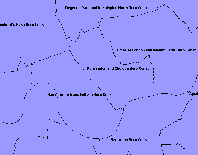
With the recent release of the OS Free Data and the up-coming election, I’ve been looking at Parliamentary Constituencies boundaries. It’s not clear from the accompanying documentation which boundary set the OS Free Data is based on, but the following image should clarify things. This is from the OS Free Data:
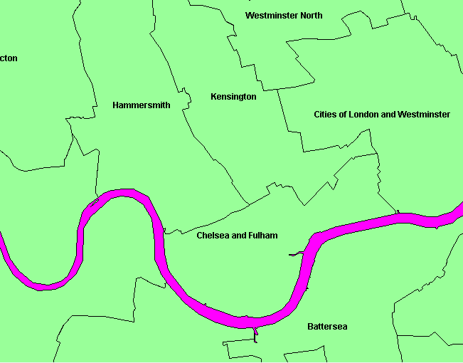
Now compare that to the PCON 2010 dataset that I obtained from the Boundary Commission:
This is the set of boundaries being used for the upcoming election as you can see that “Hammersmith and Fulham” has split into “Hammersmith” with “Fulham” being joined with “Chelsea”. This can be verified on the UK Parliament website and matched to their list of constituencies being contested in the General Election.
This means that the OS Free data is either based on the 2001 or 2008 (see National Statistics Westminster Geographies) boundary sets. It also doesn’t help that the Boundary Commission changed on 1 April 2010 from being part of the Electoral Commission to a new department called the Local Government Boundary Commission for England. This also raises the issue of the Irish political boundaries as we don’t currently have any access to them, but could make a substitute set of boundaries from postcode data.
Now that all the constituency boundaries are sorted out, we’re planning to had more electoral maps to our MapTube website, which will be at the following address:
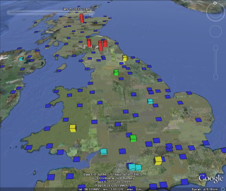
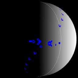
There has been quite a lot of interest about using Twitter to crowd source snow amounts, but I couldn’t help wondering how this compares to the data available from the Met Office observing network. Over the period from 20 December 2009 to 15 January 2010 I downloaded the synoptic information from the Department of Atmospheric and Environmental Sciences at the university of Albany. I then processed this using a GTS processor that I wrote, putting the decoded reports for the UK into a postgres database. Then it was a simple matter to write a Java program to interrogate this database and generate a kml file:
Although I could only get data for the hours 06:00, 12:00 and 18:00, the current snow depth will display in the KML animation until the next observation is available. This information is available for every individual hour, only not on the international feed from Albany. The data shown is snow depth on the ground in centimetres from the “sss” group in section 3 of the Synop. The height of the bars represent the depth of the snow, with colours as follows:
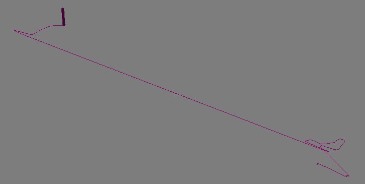
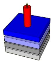
While playing around with 3DS Max 2009 for some of our GENeSIS work, I happened to notice that it’s now possible to use .net assemblies in MaxScript. My first thought was to use this for some of our agent based modelling work, but when Fabian Neuhaus asked about importing GPX files, I saw a really easy way of doing this.
The “System.Xml” assembly in .net makes parsing the GPX file extremely simple. A GPX file is nothing more than an xml file containing a list of trackpoints with a lat/lon and a time. The following script parses a GPX file and generates an animation of a box following a spline which follows the GPS track:
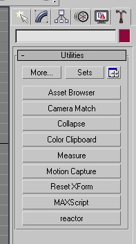
In order to use this, you have to run the script from the MaxScript rollout on the Utilities menu (click the hammer on the right hand side). Then click the “MaxScript” and “Run Script”. Point the file dialog to the file dowloaded from above and it should run.
The script creates a rollout window which allows you to browse for a GPX file to upload. After this is done, the file will be imported, resulting in an “Import Successful” message.
The only problems you might get are to do with the format of time recorded by the GPS in the track. If the import refuses to work, then you might need to change the time format as indicated by the comments in the MaxScript file.
One other thing worth mentioning is that the lat and long coordinates have been multiplied by 1000 in order to cope with a lack of granularity in Max. After producing this version of the script which loads data in the WGS84 coordinate system, I then created another version which reprojects the data into the OSGB36 system that Ordnance Survey uses in the UK. This means that we can match up the GPS tracks in Max with our own data on building footprints which comes from Ordnance Survey.
For movies showing the animated GPX tracks, have a look at the Urban Tick website:
John Conway’s “Game of Life” was one of the first things I ever wrote in Java, back in the days when we were using 1.1. This is a slight variation on the traditional 2D view, where the alife simulation is wrapped around a spinning globe. The results are shown below, along with the link to the web page containing the applet.
I’ve defined my axes with x to the right, z up and y into the screen. This is slightly unusual, but maps to the ground plane which was originally XZ.
for z=0 to numZ-1
    for x=0 to numX-1
          ax=x/numX*2.0*PI-PI;
          az=z/numZ*PI-PI/2;
          cx=radius*cos(az)*sin(ax);
          cy=radius*cos(az)*cos(ax);
          cz=radius*sin(az);
          coords[x][z]=new Point3D(cx,cy,cz);
The mesh of points can be wrapped around in the x direction, but not Z, so we need an extra line of points at the South pole. I’ve also taken the radius to be 1.0 as using the unit sphere simplifies a lot of the graphics calculations that follow.
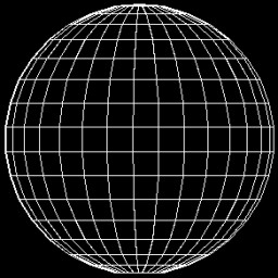
This gives you the following result:
Planet Mesh
Step 2 – Spin the World
Next I added an animation thread that increments ‘A’, the angle of rotation of the planet. In the rendering code for the mesh I rotate the points to spin the planet around the poles. The interesting thing here is that you don’t need the Y coordinate as there’s no projection, so that saves a few operations.
The back faces have been removed by using the direction between the surface normal and the viewer. Any face pointing away from the viewer is not drawn.
Step 3 – Add the Game of Life Simulation
I already had an implementaion of this in Java, so I just pulled it into the project. The following wikipedia article contains everything you could every need to know about Conway’s Game of Life:
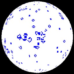
Then it’s just a case of running the ALife simulation and linking the output to the cells in the planet mesh. The grid used for the Game of Life simulation and the mesh making up the planet are the same size, so there is a simple one to one relationship.
Game of Life Planet
Step 4 – Lights
To improve the realism, I added some lighting using Lambert’s cosine rule. The direction of the light is [-1.0, 0.0, 0.0] which makes the intensity calculation straightforward. The light is assumed to be far enough away that the direction of the light is constant over the whole object. The planet is a unit sphere centred on the origin, so the normal to the surface patch is just a ray through the origin and the centre of the patch. I’ve actually taken the top left corner to save having to calculate the centre point, but it doesn’t make much difference to the effect.
According to Lambert’s cosine rule, the intensity of the patch is proportional to the cosine of the angle between the surface normal and the light. We use the dot product of the two vectors to get the cosine of the acute angle between them. As both vectors are already normalised beforehand, we don’t have to normalise them ourselves.
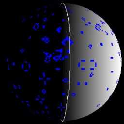
In this view, any game of life cell that is ‘on’ is drawn in blue, while any that are ‘off’ are white. The white colour uses the diffuse lighting while the blue is drawn as emissive so you can see the patterns as they go around the dark side of the globe. I’ve also added a line at the 0 and 180 degree longitude positions so you can see the planet rotating.
Here is an image of a “Gosper Glider Gun” about to shoot gliders at itself from around the other side of the planet. The applet link below contains a number of the more common patterns.
The mapping of the life grid to the planet mesh could do with some improvement. Anything moving east or west maps around the sphere correctly, but anything moving through the north pole reappears at the south and vice-versa. There are better ways to map grids onto spheres, but that’s for next time. I also have an erosion-based model that I wrote a long time ago to create realistic looking land and water masses, which this was was originally intended for.
It’s actually a stacked bar chart rather than a traditional population pyramid, but the image below shows male/female population by age for all the output areas in England. The red thematic overlay is total population for every OA, which can be clicked to get the age group breakdown shown in the popup window.
Clickable Age Map
This map is a variation on the original clickable OAC map and was built using a new version of the GMapCreator which contains the clickable technology. Traditionally, maps like this have been built using a server and database to translate the click on the client into a geographic area using point in polygon and then sending the query data back to the client. This method doesn’t scale when you have limited server resources and are looking to handle high numbers of hits, for example with the Mood Maps that we’ve been doing recently. An alternative solution is to build feature coded tiles and let the client handle most of the work displaying the data. Using this system, there is a second set of tiles, one of which the client downloads when the user clicks on a point. This allows the client to work out which feature has been clicked and request the data for that area as an xml file.
The hard part is designing a system which can allow people to design the popup window without having to resort to programming. In the example above, the graph was created using Google Charts via the GMapCreator’s user interface. All that was needed was to choose the data fields from a list and to select the chart type. The URI string to create the chart comes from an xslt transform applied to the xml data. This transform is automatically created by the GMapCreator interface, which also allows the rest of the popup window to be designed using a simple html editor.
This is one of those things that’s obvious once you know it, but I’ve often found myself developing code for tiled maps, but without a connection to the Internet. Often, I just want a quick check to see if the tiles are rendered correctly, so I don’t need the background map.
The obvious solution is to create an OpenLayers page with your custom tiles as the base layer. The javascript that makes OpenLayers work can be served locally, unlike the Google API, so by only having one layer of locally served tiles, you don’t need an Internet connection.
The html pattern follows the OpenLayers ‘howto’ guide and uses a custom TMS layer as follows:
var googlecustom=new OpenLayers.Layer.TMS(“Test”,http://www.casa.ucl.ac.uk/googlemaps/,{ ‘type’: ‘png’, ‘isBaseLayer’: true, ‘getURL’: TMSCustomGetTileURL });
The ‘TMSCustomGetTileURL’ returns the tile url based on the x, y and z value in whatever format you are storing tiles in. For this project, it was the keyhole string format.
OpenLayers map showing data from the BBC Look North Recession mood map using dynamic tile creation
The image above was taken from a prototype system using C# and SQL Server 2008 to generate tiles dynamically from data stored in a CSV file at a URL.
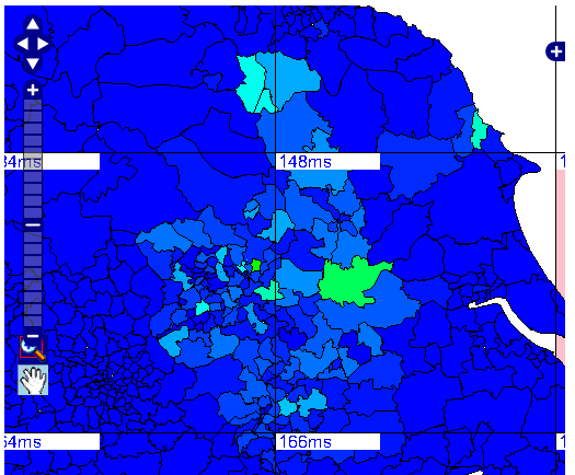
MapTube was 1 year old last week and to celebrate we have released an addition which allows you to change the background map to OpenLayers and OpenStreetMap.
Google and OpenLayers Toggle
The blue ‘G’ and the greyed out OpenLayers icon toggle the API between Google and OpenLayers. On the OpenLayers view, the basemaps can be the Mapnik, Osmarender or the Cycle Map layers which are all based on OpenStreetMap data. In addition to this, the OpenLayers API can also use the standard Google tiles as the basemap.
When creating a link to a map, the API currently in use is encoded into the URL when the ‘link to this map’ option is used. This shows up in the URL’s parameter list as “m=ol” for OpenLayers or “m=gm” for Google. For organisations where publishing links to Google Maps is a problem, this provides an open source alternative.
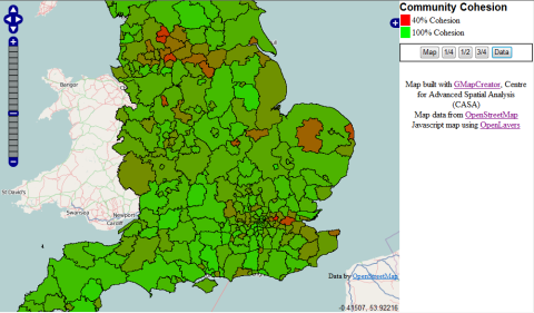
It’s actually very easy to get data from a shapefile onto OpenStreetMap using OpenLayers and the GMapCreator. The example below shows the social cohesion data from Mark Easton’s BBC blog
This page was generated using the GMapCreator and a custom template that I created for OpenLayers. The resulting map page could be completely Google free if required, but this one includes the Google map, satellite, hybrid and terrain layers as options, along with the OpenStreetMap Mapnik and Osmarender base layers.
The prototype GMapCreator template can be downloaded from the following link (right click on it and use ‘save as’ to save the file):
The file is loaded into the GMapCreator from the ‘Edit’ menu and the ‘Use Custom HTML Template’ option. All suqsequent maps will then use this template until the option is turned off.